- What changed in Version 2.0?
- Why do the variable names not match the CPS documentation from the Census?
- Which wage variable should I use?
- What weight variable should I use?
- When should I not use imputed wages?
- How do I calculate the standard errors in the CPS ORG?
Version 2.0
Version 2.0 represented a major overhaul of the CEPR CPS ORG Extract . We made a minor coding corrections to a number of variables, and dropped some variables from our extract. A full list is in the changelog at the end of the master program.
The biggest change is that we now use the Basic CPS data as the sole source for our extract from 1994 to the present. Previously we used NBER’s MORG extract as the underlying source for our extract from 1979-2002, while merging some variables from the Basic CPS into the NBER extract. With this update, we continue to use the NBER MORG extract for 1979-1993, but from 1994-present, we use the raw CPS Basic data directly from the Census.
With this update, we also updated the version of the NBER MORG for 1979-1993 to use the most recent available version of the NBER extract (accessed July 2014).
We also made significant changes to our wage variables. Most importantly, we went from carrying over 25 hourly wage variables to carrying just six. These six variables are wage1, wage2, wage3, wage4, rw, and rw_ot. We believe these variables are more straight-forward and do a better job of measuring overtime, tips, commissions, and bonuses (otc) for hourly workers.
Full details on wage variables are available in cepr_org_wages.do.
Briefly, wage1 is hourly earnings for workers paid by the hour; it excludes otc; and is available only for hourly workers.
wage2 is the usual hourly earnings, including otc, for nonhourly workers; and is available only for nonhourly workers.
wage 3 combines the usual hourly earnings for hourly workers (excluding otc) in wage1, and nonhourly workers (including otc) in wage2; wage3 is available for all workers and attempts to match the NBER’s recommendation for the most consistent hourly wage series from 1979 to the present.
wage4 is the usual hourly earnings, including otc for hourly and nonhourly workers. From 1994 to the present, this series uses hourly workers’ reported usual amounts of overtime, tips, commissions, and bonuses in order to estimate a wage for hourly workers that includes otc. From 1979 to 1993, this series attempts to estimate otc for hourly workers based on differences between weekly pay and the implied weekly pay at usual hours and straight pay. We do not place great faith in the wage4 series before 1994.
(The names wage1, wage2, wage3, and wage4 are borrowed from Economic Policy Institute terminology.)
We retained a slightly modified version of the rw variable, which is based on wage3 with a number of adjustments. First, rw converts hourly wages to constant 2014 dollars using the CPI-U-RS. Second, for workers who report a top-coded weekly earnings, we assign our estimate of the mean above the top-code, rather than the top-coded value, in order to calculate hourly earnings; our procedure uses a lognormal approximation and is applied separately by gender. (See cepr_org_topcode_lognormal.do and cps_basic_topcode_lognormal.do). We do not adjust earnings for the very small number of hourly workers whose hourly pay is top-coded.) Third, rw includes respondents who report that their weekly “hours vary.” For these workers, we use reported hourly pay or, if necessary, weekly pay together with an imputed usual weekly hours; for details, see cepr_basic_hours.do. Finally, we trim observations where the real 1989 hourly wage is below $0.50 or above $200. (For a longer, somewhat dated, discussion of the top-coding, “hours vary,” and trimming procedures, see this 2003 paper.)
rw_ot is based on wage4 (which includes otc for all workers) and otherwise makes the same adjustments as rw.
Variable Names
Our Stata programs are the major source for information on our extracts. For the CPS ORG from 1979-1993, the programs can be found here. For the CPS ORG from 1994-on, the programs can be found here. Our Stata code show the changes we made to the original raw CPS variables in order to create our extract.
Wage Variable
The CEPR preferred wage variable is rw_ot when an analysis uses only data from 1994 to the present and rw when an analysis includes data before and after 1994. Both of these variables are converted to the most recent dollars using the CPI-U-RS.
For a full discussion of wage variables, see the 2003 paper by John Schmitt, Creating a Consistent Hourly Wage Series from the Current Population Survey’s Outgoing Rotation Group, 1979-2002.
Weight Variable
You should use the orgwgt variable. If you use frequency weights, divide orgwgt by 12 and round to the nearest whole number [ex: gen weight=round(orgwgt/12,1).
Imputed Wages
See Hirsch & Schumacher (2004) for a thorough discussion. But, in general, you shouldn’t use imputed wages if you’re determining wage differentials based on variables that are not included as match criterion in the Census hot deck. Here are the characteristics included in the hot deck: gender, age, race, education, occupation, hours worked, and receipt of overtime, tips, or commissions. “If the attribute under study is not used as a census match criterion in selecting a donor, wage differential estimates (with or without controls) are biased toward zero” (Hirsch & Schumacher 2004, p. 691). Some notable characteristics not included in the hot deck are union status, industry, and public sector.
Calculating Standard Errors
The CPS is not a random sample of U.S. households –it is a “multistage stratified sample.” As a result, the procedures that statistical packages usually use to calculate standard errors will produce estimates that are systematically lower than they should be. (See Davern, Jones, Lepkowski, Davidson, and Blewett, 2007, LINK: http://www.jstor.org.proxyau.wrlc.org/stable/29773307, and Ludington, 1992, LINK:http://www.amstat.org/Sections/Srms/Proceedings/papers/1992_127.pdf, for example.)
Statistical packages (such as Stata) sometimes have procedures that take the survey design into account in order to produce more accurate estimates of standard errors. Unfortunately, the Census Bureau does not release the information about the CPS stratification method that is needed to use these procedures.
Several researchers, however, have developed procedures that can be used to approximate key features of the CPS design and allow the use of Stata (and presumably other statistical package’s) survey design routines. (Our procedure, below, is based on recommendations from Austin Nichols LINK:http://www.stata.com/statalist/archive/2008-04/msg00444.html.)
Beginning with version 1.8 of the CEPR CPS ORG extracts, for survey years from 2006 to the present, we have included variables that can be used in conjunction with the Stata svy commands to calculate more accurate standard errors than those produced by the usual procedures that do not take the CPS design into account.
The two new variables are:
cbsasz: categorical variable to identify Metropolitan Area size
cmsacode: Consolidated Statistical Area code which identifies 30 metropolitan areas
Using the following Stata code together with Stata’s svy commands will improve the accuracy of CPS standard errors:
egen psu=group(cbsasz cmsacode)
svyset [pw=orgwgt], strat(cbsasz) psu(psu)
Here is an example using data from the 2012 ORG extract. First, we calculate the weighted mean real wage for men age 16-64, without taking the CPS design into account:
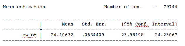
. mean rw_ot [aw=orgwgt] if female==0 & (16<=age & age<=64)
Next, we perform the same calculation allowing for the survey design using Stata’s svy command:
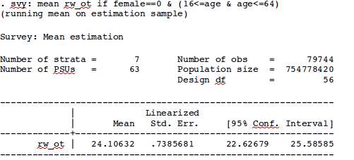
In both cases, the mean wage is identical: $24.11. But, the standard error using the canned procedure yields a standard error ($0.06) that is one-twelfth of the standard error calculated after taking the survey design into account ($0.74).
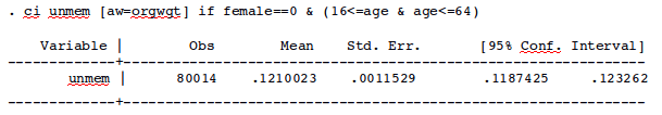
Here is another example, using a binary variable for union membership for the same population. The variable unmem takes the value 1 if the respondent is a union member, 0 if the respondent is currently working but is not a union member.
Using the standard ci command, without factoring in the survey design:
Using the proportion command and taking the survey design into account:
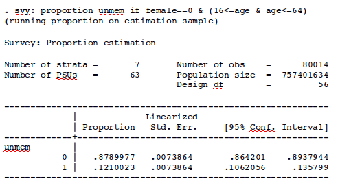
Once again, the estimated union membership share is identical across the two calculations (0.121 or 12.1 percent), but the standard error is much larger after adjusting for the survey design (0.007 versus 0.001).